A Framework to Understand DP#
This resource introduces differential privacy from the perspective of the OpenDP programming framework. No prior knowledge is assumed of differential privacy (DP), but you will likely still find this resource useful for understanding DP even if you already have a background in DP. Prior knowledge in basic probability, like random variables, will be useful.
Assume we have a vector dataset \(u\) where each record contains sensitive information about a different individual.
[2]:
# u is a small vector dataset with contributions from:
#   [Alice, Jane, John, Jack, ...]
u = [12,    10,   8,    7,       ]
We can use differential privacy to collect measurements (statistics such as means and histograms) on this dataset, without revealing information about specific individuals.
Distance Between Datasets - Adjacency#
An adjacent dataset is any dataset that differs from our dataset by a single individual. Returning to our vector dataset example, assume our dataset \(u\) has one record that contains information about a person, Alice. Then one adjacent dataset \(v\) would contain every row in \(u\) except for the row with Alice’s information.
[3]:
# v is one (of many) datasets that are adjacent to u
#   [Jane, John, Jack, ...] (without Alice!)
v = [10,   8,    7,       ]
You can construct other datasets adjacent to \(u\) by dropping a different row or adding a new row. When one person may contribute up to \(k\) rows, adjacent datasets differ by up to \(k\) additions and removals.
The number of additions/removals between any two datasets is equivalent to the cardinality of the symmetric difference between the multisets \(u\) and \(v\). We call this metric the symmetric distance.
And in code:
[4]:
def d_SymmetricDistance(u, v):
    """symmetric distance between multisets u and v"""
    # NOT this, as sets are not multisets. Loses multiplicity:
    # return len(set(u).symmetric_difference(set(v)))

    from collections import Counter
    u, v = Counter(u), Counter(v)
    # indirectly compute symmetric difference via the union of asymmetric differences
    return sum(((u - v) + (v - u)).values())


# compute the symmetric distance between our two example datasets:
d_SymmetricDistance(u, v)
[4]:
1
\(d_{\mathrm{Sym}}(\{12, 10, 8, 7\}, \{10, 8, 7\}) = |\{12, 10, 8, 7\} \triangle \{10, 8, 7\}| = |\{12\}| = 1\)
If the second dataset \(v\) were to differ from \(u\) by changing the 12 to 10, then we would still count the multiplicity of 10:
\(d_{\mathrm{Sym}}(\{12, 10, 8, 7\}, \{10, 10, 8, 7\}) = |\{12, 10, 8, 7\} \triangle \{10, 10, 8, 7\}| = |\{12, 10\}| = 2\)
In practice, we never directly compute these distances. In order to apply differentially private methods, you need to establish an upper bound on the distance between adjacent datasets. For example, if each individual person may affect up to five records in the dataset, then setting a distance \(d_in = 5\) allows us to ensure individual-level privacy.
For instance, in the vector dataset example, it was stipulated that each element contains sensitive information about a different individual. This statement implies that the symmetric distance between adjacent datasets, where one individual is added or removed, is at most one. That is, for any choice of datasets \(u\) and \(v\) such that \(u\) is adjacent to \(v\) (denoted \(u \sim_{\mathrm{Sym}} v\)), we have that \(d_{\mathrm{Sym}}(u, v) \leq 1\).
Before moving on, there are some trivial generalizations. A dataset need not be a vector, it could be a dataframe or any other collection with a concept of records. There are also other dataset metrics aside from SymmetricDistance (used for unbounded DP), such as ChangeOneDistance (used for bounded DP). There are also variations of metrics that are sensitive to data ordering, metrics for describing distances between graphs, and more!
You should now have a sense for what an adjacent dataset means, how dataset distances work, and an intuitive understanding of the symmetric distance metric.
Distance Between Distributions - Divergence#
You can think of a measurement \(M(\cdot)\) as a differentially private statistic. Measurements are described by random variables (RVs), that is, they sample from noise distributions. The outputs of a measurement are realizations of a random variable that follow a known probability distribution. Measurements only have one input: a dataset; other parameters are fixed when the measurement is constructed. For context, a Laplace RV has parameters for shift and scale. This section describes how to measure distance between the distributions of measurements on adjacent datasets.
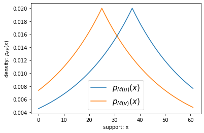
A common measurement is the Laplace DP sum, which is a sample from the Laplace distribution centered at the dataset sum with a fixed noise scale. The following plot compares the distribution of the DP sum on dataset \(u\) with the distribution of the DP sum on dataset \(v\), when the noise scale is fixed to 25.
[8]:
import numpy as np
import matplotlib.pyplot as plt

scale = 25

# while in this case the support theoretically includes all reals,
#     we only bother plotting part of the support
support = np.arange(sum(v) - scale, sum(u) + scale)

def rv_M(x):
    """returns a random variable, M(x)"""
    from scipy.stats import laplace
    return laplace(loc=sum(x), scale=scale)

def plot_pdfs(u, v, output_domain):
    plt.plot(output_domain, rv_M(u).pdf(output_domain), label="$p_{M(u)}(x)$") # type: ignore
    plt.plot(output_domain, rv_M(v).pdf(output_domain), label="$p_{M(v)}(x)$") # type: ignore
    plt.ylabel('density: $p_{RV}(x)$')
    plt.xlabel('support: x')
    plt.legend(prop={'size': 15})
plot_pdfs(u, v, support)

We are interested in the greatest divergence, a measure of the dissimilarity of these two distributions. While divergences are not necessarily distances, we informally refer to them as distances. A common measure of divergence is based on the log ratio of probabilities:
In this equation we define the distance between the RVs of \(M(u)\) and \(M(v)\) to be the maximum divergence among all possible subsets of the support.
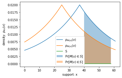
For our DP sum with Laplacian noise example, the output domain of \(M(\cdot)\) is the set of all real numbers, \(\mathbb{R}\). In the plot below, I illustrate this equation for one randomly chosen subset \(S\) of the output domain:
[20]:
def plot_S(u, v, S):
    """draw the probability regions spanned by S"""
    plt.fill_between(S, rv_M(u).pdf(S), label="$\\Pr[M(u) \\in S]$", alpha=.4) # type: ignore
    plt.fill_between(S, rv_M(v).pdf(S), label="$\\Pr[M(v) \\in S]$", alpha=.4) # type: ignore
    plt.plot([np.min(S), np.max(S)], [0, 0], label="S")
    plt.legend()

# re-run this notebook to see different choices of S
S = np.arange(*sorted(np.random.choice(support, size=2, replace=False)))

plot_pdfs(u, v, support)
plot_S(u, v, S)

The area of the blue region is the probability that \(M(u)\) is in \(S\)… and similarly the area of the orange region is \(\Pr[M(v) \in S]\).
[21]:
def divergence_over_S(u, v, S):
    """prints the Divergence(M(u), M(v)) over some interval S, assuming M(x) = Laplace(sum(x), scale)"""

    # integrate over both regions
    lower, upper = np.min(S), np.max(S)
    pr_Mu_in_S = rv_M(u).cdf(upper) - rv_M(u).cdf(lower) # blue
    pr_Mv_in_S = rv_M(v).cdf(upper) - rv_M(v).cdf(lower) # orange

    print("area of blue region:  ", pr_Mu_in_S)
    print("area of orange region:", pr_Mv_in_S)
    print("divergence for this S:", np.abs(np.log(pr_Mu_in_S / pr_Mv_in_S)))
divergence_over_S(u, v, S)
area of blue region:   0.2276049566440389
area of orange region: 0.14083816706408814
divergence for this S: 0.4799999999999992
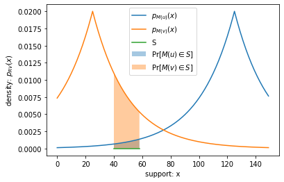
This shows the divergence between the RVs of \(M(u)\) and \(M(v)\) for one choice of S, but keep in mind that \(D_{\mathrm{MaxDivergence}}(M(u), M(v))\) is the greatest divergence over any choice of \(S\). Intuitively, the divergence between the RVs of \(M(u)\) and \(M(v)\) for the same \(S\) must increase if Alice made a greater contribution to the statistic:
[22]:
# hypothetical: what if Alice's contribution was 100, instead of 12?
u_prime = [100, *u[1:]]
divergence_over_S(u_prime, v, S)

output_domain = np.arange(sum(v) - scale, sum(u_prime) + scale, 1)
plot_pdfs(u_prime, v, output_domain)
plot_S(u_prime, v, S)
area of blue region:   0.017594942096975916
area of orange region: 0.14083816706408814
divergence for this S: 2.080000000000001

As we can see, when the divergence between probability distributions is greater, we can more confidently distinguish which distribution a sample came from. These examples help to form an intuition for how the max divergence measure relates to privacy.
Moreso, the max divergence qualifies as a measure of privacy because it provides immunity from post-processing. There is no further computation that can be made on the release that will make it easier to distinguish which distribution a sample came from. That is, the divergence cannot increase after applying \(f\) to a release:
This property is the crucial distinction between measures, as discussed in this section, and metrics, as discussed in the previous section. Measurements and transformations share the same distinction.
Definition of Privacy#
Now that we have an understanding of distances between datasets, and distances between distributions, we can define the privacy of a measurement, \(M(\cdot)\):
\(M(\cdot)\) is \(\boldsymbol\epsilon\textbf{-differentially private}\) at distance \(k\) if, for every pair of datasets \(u\) and \(v\) such that \(d_{\mathrm{Sym}}(u, v) \leq k\), we have that \(D_{\mathrm{MaxDivergence}}(M(u), M(v)) \leq \epsilon\).
In this definition, we relate a dataset distance \(k\) to another distance \(\epsilon\). This \(\epsilon\) is more general than the max divergence we computed in the previous section because it is the greatest divergence over all possible choices of \(S\), and over all possible pairs of adjacent datasets \(u\) and \(v\). \(\epsilon\) is often referred to as a bound on the privacy loss of \(M(\cdot)\).
This has a very practical interpretation: Let’s say I have a dataset \(x\) for which an individual user can contribute at most \(k\) rows, and a statistic \(M(\cdot)\) that is \(\epsilon\)-DP when user contribution is at most \(k\). By the DP guarantee, it is proven that the influence of any one individual on the data release induces a divergence no greater than \(\epsilon\). Thus, assuming a reasonably small choice of \(\epsilon\), the individual’s participation in the statistical release is kept private, because their influence on the data release is at most \(\epsilon\)-distinguishable.
If you have some background in differential privacy you may be more familiar with a definition of privacy worded like this:
\(M(\cdot)\) is \(\boldsymbol\epsilon\textbf{-differentially private}\) if, for every pair of adjacent datasets \(u\) and \(v\), we have that \(\Pr[M(u) \in S] \leq e^\epsilon \cdot \Pr[M(v) \in S]\).
This is mostly equivalent, because of the way we’ve defined \(D_{\mathrm{MaxDivergence}}(M(u), M(v))\) in the previous section. However, this formulation of the definition is ambiguous about what makes a dataset adjacent. To obtain well-defined privacy guarantees, it is important to specify the dataset metric and dataset distance.
We further generalize the definition of privacy:
\(M(\cdot)\) is \((d_{in}, d_{out})\textbf{-differentially private}\) with respect to input metric \(MI\) and output measure \(MO\) if, for any choice of datasets \(u\) and \(v\) such that \(d_{MI}(u, v) \leq d_{in}\), we have that \(D_{MO}(M(u), M(v)) \leq d_{out}\).
The first definition can be reclaimed by letting \(MI\) be SymmetricDistance and \(MO\) be MaxDivergence. \(MO\) can be set to other measures of divergence to represent approximate (\(\epsilon, \delta\))-differential privacy, or zero-concentrated \(\rho\)-differential privacy. Similarly, our choice of SymmetricDistance represents unbounded DP, but we can represent bounded DP by letting \(MI\) be ChangeOneDistance.
Distance Between Aggregates - Sensitivity#
The sensitivity is the greatest amount an aggregate can change when computed on an adjacent dataset. Aggregators are typically deterministic statistics (like the sum or histogram functions), and their exact outputs are aggregates. More generally, a transformation \(T(\cdot)\) is a function from a data domain to a data domain. Aggregators are a kind of transformation in which the output domain consists of aggregates.
One example of a sensitivity metric is the AbsoluteDistance, which is used to measure the distance between scalar aggregates.
[8]:
def d_Abs(a, b):
    """absolute distance between a and b"""
    return abs(a - b)
We can use the absolute distance metric to express the sensitivity of the sum aggregator. In our vector dataset example, we know each individual can contribute at most one record. Since this record is unbounded, it can perturb the sum an arbitrarily large amount towards positive or negative infinity. This is unfortunate, because it implies that the divergence is also infinite!
In order to attain a finite sensitivity, it is customary to clamp— that is, to replace any value less than a lower bound with the lower bound, and any value greater than an upper bound with the upper bound.
[9]:
def clamped_sum_0_12(x):
    """a naive function that computes the sum, where each element is clamped within [0, 12]"""
    return sum(np.clip(x, 0, 12))
Broadly speaking, if the transformation clamps data to the interval \([L, U]\), and we know each individual contributes at most \(d_{in}\) records, then the clamped sum sensitivity (\(d_{out}\)) is
We can use this to solve for the sensitivity of \(clamped\_sum\_0\_12\), by letting \([L, U] = [0, 12]\). Thus its sensitivity is \(1 \cdot max(|0|, 12) = 12\). For any conceivable dataset \(u\), adding or removing any individual (to get some dataset \(v\)) can change the sum by at most \(12\).
Our current choice of \(u\) and \(v\) is an example that maximizes the absolute distance:
[10]:
d_Abs(clamped_sum_0_12(u), clamped_sum_0_12(v))
[10]:
12
You can even use the AbsoluteDistance as the input metric \(MI\) of a measurement \(M(\cdot)\) (see the definition of privacy). Let’s define a new function \(laplace\_noise\) to illustrate this:
[11]:
def laplace_noise(x):
    """a naive function that adds an approximation to Laplace noise"""
    return np.random.laplace(loc=x, scale=scale)
We let \(MI\) be AbsoluteDistance and \(MO\) be MaxDivergence. It can be shown that for any choice of \(u, v \in \mathbb{R}\) such that \(d_{\mathrm{Abs}}(u, v) \leq d_{in}\), and \(d_{out} = d_{in} / scale\), then:
Therefore, if the data types in this function had infinite precision, then \(laplace\_noise\) would be a measurement. Other common metrics to express sensitivities are L1Distance and L2Distance.
Definition of Stability#
Similar to how we defined the privacy of a measurement \(M(\cdot)\), we can also define the stability of a transformation, \(T(\cdot)\):
\(T(\cdot)\) is \((d_{in}, d_{out})\textbf{-stable}\) with respect to input metric \(MI\) and output metric \(MO\) if, for any choice of datasets \(u\) and \(v\) such that \(d_{MI}(u, v) \leq d_{in}\), we have that \(d_{MO}(T(u), T(v)) \leq d_{out}\).
An example is the \(clamped\_sum\_0\_12\) function from the previous section. If the data types in \(clamped\_sum\_0\_12\) had infinite precision, it would be a stable transformation where \(MI\) is SymmetricDistance and \(MO\) is AbsoluteDistance. We’ve previously shown that when \(d_{in} = 1\), the sensitivity \(d_{out} = 12\).
This stability guarantee does not carry privacy guarantees on its own, but it lets us construct building blocks that can be chained together. If the output metric \(MO\) and output domain \(DO\) of a transformation \(T(\cdot)\) conform with the input metric \(MI\) and input domain \(DI\) of a measurement \(M(\cdot)\), then it is valid to construct a new measurement \(M_{\mathrm{chained}}(\cdot) = M(T(\cdot))\). We can similarly construct a new transformation \(T_{\mathrm{chained}}(\cdot) = T_2(T_1(\cdot))\).
Notice that the output domain and metric of the \(clamped\_sum\_0\_12\) transformation conform with the input metric and domain of the \(laplace\_noise\) measurement, so we can chain these together:
[12]:
def laplace_sum(x):
    """a naive function that computes the noisy clamped sum"""
    return laplace_noise(clamped_sum_0_12(x))
Since this function was constructed by chaining a stable transformation and private measurement, it is trivial to prove that it is a private measurement (if the data types had infinite precision). The new chained measurement’s \(MI\) is SymmetricDistance, and \(MO\) is MaxDivergence, and when the dataset distance \(d_{in} = 1\), we have that \(\epsilon = d_{out} = d_{in} \cdot \max(|0|, 12) / 25 = d_{in} \cdot 0.48 = 0.48\). That is, when an individual can contribute at
most one record, the maximum observable divergence among the output distributions is \(0.48\).
Stability Maps and Privacy Maps#
A crucial takeaway from this notebook is a high-level understanding that differential privacy is a system to relate distances (\(d_{in}\) and \(d_{out}\)). If you can establish a bound on the distance to adjacent datasets \(d_{in}\) (in terms of some metric \(MI\)) then you can work out the stability or privacy properties \(d_{out}\) (in terms of some metric or measure \(MO\)) of computations made on your data.
We encapsulate this relationship between distances with one last abstraction, a map. A map is a function, associated with your computation, that computes a \(d_{out}\) for any given \(d_{in}\). Thus, if \(map(d_{in}) \le d_{out}\), then a computation is \(d_{out}\)-DP.
The stability map for the \(clamped\_sum\_0\_12\) function is as follows:
[13]:
def clamped_sum_0_12_map(d_in):
    return d_in * max(abs(0), 12)

# find the smallest d_out (absolute distance) of clamped_sum_0_12 when d_in (symmetric distance) is 1
clamped_sum_0_12_map(d_in=1)
[13]:
12
This map is just a repackaging of our previous formula for the clamped sum sensitivity, so that \(d_{in}\) can be set later. It is referred to as a stability map because stability is a more general term than sensitivity, namely a bound on on how much outputs can change as a function of input distances.
The same pattern holds for the privacy map of the \(laplace\_noise\) measurement:
[14]:
def laplace_noise_map(d_in):
    return d_in / scale

# find the smallest d_out (epsilon) of laplace_noise when d_in (absolute distance) is 12
laplace_noise_map(d_in=12)
[14]:
0.48
This time we refer to it as a privacy map, because the output distance is in terms of a privacy measure, which captures distance between output distributions (like MaxDivergence) and hence offers privacy guarantees. Now that we have the stability map for the clamped sum transformation and the privacy map for the Laplace noise measurement, we can automatically construct the privacy map for the Laplace sum measurement:
[15]:
def laplace_sum_map(d_in):
    return laplace_noise_map(clamped_sum_0_12_map(d_in))

# find the smallest d_out (epsilon) of laplace_noise when d_in (symmetric distance) is 1
laplace_sum_map(1)
[15]:
0.48
We’ve now come full-circle. In the “Distance Between Distributions” section, we computed an example divergence for one choice of \(S\). We have now indirectly computed an upper bound for that divergence of \(0.48\). You may notice that some choices of \(S\) in that section can give divergences very slightly larger than \(0.48\). This is because floating-point numbers have finite precision, so intermediate computations were subject to rounding that introduced error.
The transformation and measurement examples in this notebook are only \((d_{in}, d_{out})\)-differentially private if we assume the data types have infinite precision— and they don’t! Building transformations or measurements that have proven stability or privacy properties is nontrivial, especially if you account for finite precision in data types. This is the purpose of the OpenDP library: to help you build robust transformations and measurements with rigorous privacy properties.
