Thiel-Sen Regression#
This example demonstrates how transformation and measurement plugins can be combined to build a differentially private Theil-Sen-style regression estimator.
Note
If you actually want to use Theil-Sen in Python, don’t copy-and-paste this code.
It is already implemented by the OpenDP library: see the opendp.extras.sklearn.linear_model API reference.
The high-level flow is:
Build a user-defined transformation that pairs records and predicts response values at two cut points.
Build a user-defined measurement that privately estimates the medians of those predictions.
Postprocess the private medians into slope and intercept coefficients.
Enable plugin-related features:
>>> import opendp.prelude as dp
>>> import numpy as np
>>> from pathlib import Path
>>> dp.enable_features("contrib", "honest-but-curious")
enable_features("contrib", "honest-but-curious")
1. Pairwise Prediction Transformation#
Construct a transformation that pairs rows and predicts response values at two x-axis cut points.
>>> def pairwise_predict(data, x_cuts):
...     data = np.array(data, copy=True)[: len(data) // 2 * 2]
...     np.random.shuffle(data)
...     p1, p2 = np.array_split(data, 2)
...     dx, dy = (p2 - p1).T
...     x_bar, y_bar = (p1 + p2).T / 2
...     points = dy / dx * (x_cuts[None].T - x_bar) + y_bar
...     return points.T[dx != 0]
...
>>> def make_pairwise_predict(x_cuts, runs: int = 1):
...     return dp.t.make_user_transformation(
...         input_domain=dp.numpy.array2_domain(
...             num_columns=2, T=float
...         ),
...         input_metric=dp.symmetric_distance(),
...         output_domain=dp.numpy.array2_domain(
...             num_columns=2, T=float
...         ),
...         output_metric=dp.symmetric_distance(),
...         function=lambda x: np.vstack(
...             [
...                 pairwise_predict(x, x_cuts)
...                 for _ in range(runs)
...             ]
...         ),
...         stability_map=lambda d_in: d_in * runs,
...     )
...
pairwise_predict <- function(data, x_cuts) {
  data <- as.matrix(data)
  data <- data[seq_len(nrow(data) %/% 2L * 2L), , drop = FALSE]
  data <- data[sample(nrow(data)), , drop = FALSE]

  midpoint <- nrow(data) %/% 2L
  p1 <- data[seq_len(midpoint), , drop = FALSE]
  p2 <- data[midpoint + seq_len(midpoint), , drop = FALSE]

  dx <- p2[, 1L] - p1[, 1L]
  dy <- p2[, 2L] - p1[, 2L]
  x_bar <- (p1[, 1L] + p2[, 1L]) / 2L
  y_bar <- (p1[, 2L] + p2[, 2L]) / 2L

  predicted_points <- sapply(
    x_cuts,
    function(x_cut) dy / dx * (x_cut - x_bar) + y_bar
  )
  predicted_points[dx != 0L, , drop = FALSE]
}

make_pairwise_predict <- function(
  input_domain,
  input_metric,
  x_cuts,
  runs = 1L
) {
  make_user_transformation(
    input_domain = input_domain,
    input_metric = input_metric,
    output_domain = input_domain,
    output_metric = input_metric,
    function_ = function(x) {
      as.data.frame(
        do.call(
          rbind,
          replicate(runs, pairwise_predict(x, x_cuts), simplify = FALSE)
        )
      )
    },
    stability_map = function(d_in) d_in * runs
  )
}
then_pairwise_predict <- to_then(make_pairwise_predict)
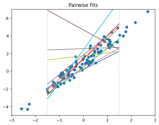
The figure below shows the intuition behind the pairwise prediction step: each sampled pair induces a line, and the mechanism records the predicted y-values where those lines cross two fixed x-axis cut points.
Python code to generate this figure
>>> def render_pairwise_visualization():
...     import matplotlib.pyplot as plt
...     pairwise_plot_path = Path(__file__).with_name(
...         "theil-sen-pairwise-fits.png"
...     )
...     pairwise_plot_x_cuts = np.array([-1.5, 1.5])
...     pairwise_plot_x = np.linspace(-2.5, 2.5, 12)
...     pairwise_plot_y = 2 * pairwise_plot_x + 1
...     pairwise_plot_data = np.column_stack(
...         [pairwise_plot_x, pairwise_plot_y]
...     )
...     p1, p2 = np.array_split(pairwise_plot_data, 2)
...     fig, ax = plt.subplots(figsize=(7, 4.5))
...     ax.scatter(
...         pairwise_plot_data[:, 0],
...         pairwise_plot_data[:, 1],
...         color="black",
...         s=20,
...     )
...     for point_1, point_2 in zip(p1, p2):
...         slope = (point_2[1] - point_1[1]) / (
...             point_2[0] - point_1[0]
...         )
...         intercept = point_1[1] - slope * point_1[0]
...         ax.plot(
...             pairwise_plot_x,
...             slope * pairwise_plot_x + intercept,
...             color="#7a9e9f",
...             alpha=0.45,
...         )
...         predicted = slope * pairwise_plot_x_cuts + intercept
...         ax.scatter(
...             pairwise_plot_x_cuts,
...             predicted,
...             color="#bc4b51",
...             s=28,
...             zorder=3,
...         )
...     for x_cut in pairwise_plot_x_cuts:
...         ax.axvline(
...             x_cut,
...             color="#2c4c7c",
...             linestyle="--",
...             linewidth=1,
...         )
...     ax.set_title("Pairwise Predictions at Fixed Cut Points")
...     ax.set_xlabel("x")
...     ax.set_ylabel("y")
...     fig.tight_layout()
...     fig.savefig(pairwise_plot_path, dpi=150)
...     plt.close(fig)
...
2. Private Median Subroutine#
Construct a measurement that privately estimates the median prediction at each cut point.
>>> def make_select_column(j):
...     return dp.t.make_user_transformation(
...         input_domain=dp.numpy.array2_domain(
...             num_columns=2, T=float
...         ),
...         input_metric=dp.symmetric_distance(),
...         output_domain=dp.vector_domain(
...             dp.atom_domain(T=float)
...         ),
...         output_metric=dp.symmetric_distance(),
...         function=lambda x: x[:, j],
...         stability_map=lambda d_in: d_in,
...     )
...
>>> def make_private_percentile_medians(
...     output_measure, y_bounds, scale
... ):
...     m_median = dp.m.then_private_quantile(
...         output_measure,
...         candidates=np.linspace(*y_bounds, 100),
...         alpha=0.5,
...         scale=scale,
...     )
...     return dp.c.make_composition(
...         [
...             make_select_column(0)
...             >> dp.t.then_drop_null()
...             >> m_median,
...             make_select_column(1)
...             >> dp.t.then_drop_null()
...             >> m_median,
...         ]
...     )
...
make_select_column <- function(input_domain, input_metric, j) {
  make_user_transformation(
    input_domain = input_domain,
    input_metric = input_metric,
    output_domain = vector_domain(atom_domain(.T = f64)),
    output_metric = symmetric_distance(),
    function_ = function(x) x[, j],
    stability_map = function(d_in) d_in
  )
}
then_select_column <- to_then(make_select_column)

make_private_medians <- function(
  input_domain,
  input_metric,
  output_measure,
  y_bounds,
  scale
) {
  candidates <- seq(y_bounds[[1L]], y_bounds[[2L]], length.out = 100L)
  column_space <- c(input_domain, input_metric)
  first_median <- column_space |>
    then_select_column(1L) |>
    then_drop_null() |>
    then_private_quantile(
      output_measure = output_measure,
      candidates = candidates,
      alpha = 0.5,
      scale = scale
    )
  second_median <- column_space |>
    then_select_column(2L) |>
    then_drop_null() |>
    then_private_quantile(
      output_measure = output_measure,
      candidates = candidates,
      alpha = 0.5,
      scale = scale
    )

  make_composition(c(first_median, second_median))
}
then_private_medians <- to_then(make_private_medians)
3. Assemble the Mechanism#
Combine the transformation, private medians, and postprocessing into a single measurement.
>>> def make_private_theil_sen(
...     output_measure, x_bounds, y_bounds, scale, runs=1
... ):
...     x_cuts = x_bounds[0] + (
...         x_bounds[1] - x_bounds[0]
...     ) * np.array([0.25, 0.75])
...     p_inv = np.linalg.inv(
...         np.vstack([x_cuts, np.ones_like(x_cuts)]).T
...     )
...     return (
...         make_pairwise_predict(x_cuts, runs)
...         >> make_private_percentile_medians(
...             output_measure, y_bounds, scale
...         )
...         >> (lambda ys: p_inv @ ys)
...     )
...
>>> x_bounds = (-3.0, 3.0)
>>> y_bounds = (-10.0, 10.0)
>>> meas = make_private_theil_sen(
...     dp.max_divergence(), x_bounds, y_bounds, scale=1.0
... )
>>> meas.map(1)
2.0
make_private_theil_sen <- function(
  input_domain,
  input_metric,
  output_measure,
  x_bounds,
  y_bounds,
  scale,
  runs = 1L
) {
  x_cuts <- x_bounds[[1L]] + (x_bounds[[2L]] - x_bounds[[1L]]) * c(0.25, 0.75)
  p_inv <- solve(cbind(x_cuts, 1L))

  c(input_domain, input_metric) |>
    then_pairwise_predict(x_cuts, runs) |>
    then_private_medians(output_measure, y_bounds, scale) |>
    then_postprocess(
      function(ys) as.vector(p_inv %*% as.numeric(unlist(ys))),
      .TO = "Vec<f64>"
    )
}
then_private_theil_sen <- to_then(make_private_theil_sen)

x_bounds <- c(-3.0, 3.0)
y_bounds <- c(-10.0, 10.0)
input_space <- c(
  user_domain(
    identifier = "DataFrame2Domain",
    member = function(x) is.data.frame(x) && ncol(x) == 2L
  ),
  symmetric_distance()
)
meas <- input_space |>
  then_private_theil_sen(max_divergence(), x_bounds, y_bounds, scale = 1.)
meas(d_in = 1L)
4. Run a Private Release#
Apply the measurement to synthetic data to obtain private regression coefficients.
>>> np.random.seed(1)
>>> def f(x):
...     return x * 2 + 1
...
>>> x = np.random.normal(size=100, loc=0, scale=1.0)
>>> y = f(x) + np.random.normal(size=100, loc=0, scale=0.5)
>>> slope, intercept = meas(np.stack([x, y], axis=1))
>>> round(float(slope), 6), round(
...     float(intercept), 6
... )
(..., ...)
f <- function(x) x * 2L + 1L

x <- rnorm(100L)
y <- f(x) + rnorm(100L, sd = 0.5)
private_data <- data.frame(x = x, y = y)
meas(arg = private_data)
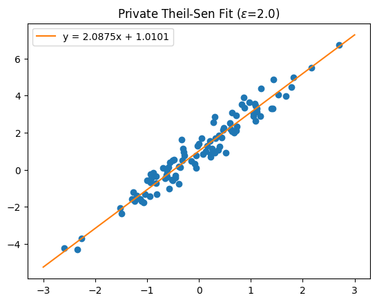
The original notebook also visualized the resulting private fit:
Python code to generate this figure
>>> def render_private_fit_visualization():
...     import matplotlib.pyplot as plt
...     private_fit_plot_path = Path(__file__).with_name(
...         "theil-sen-private-fit.png"
...     )
...     fig, ax = plt.subplots(figsize=(7, 4.5))
...     ax.scatter(
...         x,
...         y,
...         color="black",
...         s=14,
...         alpha=0.7,
...         label="synthetic data",
...     )
...     plot_x = np.linspace(x.min(), x.max(), 200)
...     ax.plot(
...         plot_x,
...         f(plot_x),
...         color="#2c4c7c",
...         linewidth=2,
...         label="true fit",
...     )
...     ax.plot(
...         plot_x,
...         slope * plot_x + intercept,
...         color="#bc4b51",
...         linewidth=2,
...         label="private fit",
...     )
...     ax.set_title("Private Theil-Sen Regression Fit")
...     ax.set_xlabel("x")
...     ax.set_ylabel("y")
...     ax.legend()
...     fig.tight_layout()
...     fig.savefig(private_fit_plot_path, dpi=150)
...     plt.close(fig)
...