Aggregation: Quantile

This notebook explains techniques for releasing differentially private quantiles. Unlike counts and sums, the quantile can change by a large amount when one person contributes their data.

from statistics import median

# Given bounds of 0 and 100...
L, U = 0, 100

# ...and elements of x are at the bounds...
x = [L, U] * 50

# ...the median changes from 50 to 100 when one individual is added
print('before:', median(x))
print('after:', median(x + [U]))

before: 50.0
after: 100

Even when the datasets are always non-empty, the sensitivity of \((U - L) / 2\) is too large for additive noise mechanisms to be suitable for estimating quantiles.

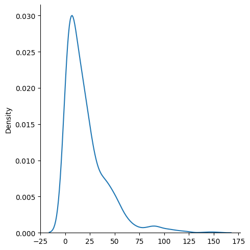
Instead of using this dataset of extremes, we’ll demonstrate differentially private techniques with a more realistic skewed dataset sampled from \(\mathrm{Exponential}(\lambda=20)\).

# privacy settings for all examples:
max_contributions = 1
epsilon = 1.

import numpy as np
data = np.random.exponential(20., size=1000)
bounds = 0, 100 # a best guess!

import seaborn as sns
sns.displot(data, kind="kde");

# true quantiles
quartiles = [0.25, 0.5, 0.75]
true_quantiles = np.quantile(data, quartiles)
true_quantiles.tolist()

[5.800778225846171, 14.663246151408615, 28.49926270360073]

---

Any functions that have not completed the proof-writing and vetting process may still be accessed if you opt-in to “contrib”. Please contact us if you are interested in proof-writing. Thank you!

import opendp.prelude as dp
dp.enable_features("contrib")

Quantile via Exponential Mechanism

Individual quantiles can be estimated via private_quantile, which uses the exponential mechanism.

context = dp.Context.compositor(
    data=data,
    privacy_unit=dp.unit_of(contributions=1),
    privacy_loss=dp.loss_of(epsilon=1.),
    split_evenly_over=3,
)

candidates = list(range(*bounds))

def release_quantile(alpha):
    query = context.query().drop_null().private_quantile(dp.max_divergence(), candidates, alpha)
    return query.release()

[release_quantile(alpha) for alpha in quartiles]

[6.0, 15.0, 28.0]

This is equivalent to the following, in the lower-level framework API:

input_space = dp.vector_domain(dp.atom_domain(T=float)), dp.symmetric_distance()


def make_expo_quantiles(alphas, d_in, d_out):
    t_pre = dp.t.make_drop_null(*input_space)
    def make_from_scale(scale):
        return dp.c.make_composition([
            dp.m.make_private_quantile(*t_pre.output_space, dp.max_divergence(), candidates, alpha, scale)
            for alpha in alphas
        ])
    return dp.binary_search_chain(make_from_scale, d_in=d_in, d_out=d_out)


m_expo_quantile = make_expo_quantiles(quartiles, d_in=1, d_out=1.)
m_expo_quantile(data)

[6.0, 15.0, 28.0]

Quantile via Histogram

Estimating the cumulative distribution function (CDF) performs better than releasing individual quantiles when you want to release a large number of quantiles. The CDF can be estimated by simply releasing a histogram.

The basic procedure for estimating an \(\alpha\)-quantile is as follows:

1. bin the data, and count the number of elements in each bin privately

2. divide the counts by the total to get the probability density of landing in each bin

3. sum the densities while scanning from the left until the sum is at least \(\alpha\)

4. interpolate the bin edges of the terminal bin

def make_hist_quantiles(alphas, d_in, d_out, num_bins=500):

    edges = np.linspace(*bounds, num=num_bins + 1)
    bin_names = [str(i) for i in range(num_bins)]

    def make_from_scale(scale):
        return (
            input_space >>
            dp.t.then_drop_null() >>
            dp.t.then_find_bin(edges=edges) >> # bin the data
            dp.t.then_index(bin_names, "0") >> # can be omitted. Just set TIA="usize", categories=list(range(num_bins)) on next line:
            dp.t.then_count_by_categories(categories=bin_names, null_category=False) >>
            dp.m.then_laplace(scale) >>
            # we're really only interested in the function on this transformation- the domain and metric don't matter
            dp.t.make_cast_default(dp.vector_domain(dp.atom_domain(T=int)), dp.symmetric_distance(), TOA=float) >>
            dp.t.make_quantiles_from_counts(edges, alphas=alphas)
        )

    return dp.binary_search_chain(make_from_scale, d_in, d_out)

hist_quartiles_meas = make_hist_quantiles(quartiles, max_contributions, epsilon)
hist_quartiles_meas(data)

[5.945, 14.73, 28.150000000000006]

A drawback of using this algorithm is that it can be difficult to choose the number of bins.

If the number of bins is chosen to be very small, then the postprocessor will need to sum fewer instances of noise before reaching the bin of interest, resulting in a better bin selection. However, the bin will be wider, so there will be greater error when interpolating the final answer.

If the number of bins is chosen to be very large, then the same holds in the other direction.

Estimating quantiles via the next algorithm can help make choosing the number of bins less sensitive.

Quantile via B-ary Tree

A slightly more complicated algorithm that tends to provide better utility is to privatize a B-ary tree instead of a histogram. In this algorithm, the raw counts form the leaf nodes, and a complete tree is constructed by recursively summing groups of size b. This results in a structure where each parent node is the sum of its b children. Noise is added to each node in the tree, and then a postprocessor makes all nodes of the tree consistent with each other, and returns the leaf nodes.

In the histogram approach, the postprocessor would be influenced by a number of noise sources approximately \(O(n)\) in the number of scanned bins. After this modification, the postprocessor is influenced by a number of noise sources approximately \(O(\log_b(n))\) in the number of scanned bins, and with noise sources of similarly greater magnitude.

This modification introduces a new hyperparameter, the branching factor. choose_branching_factor provides a heuristic for the ideal branching factor, based on information (or a best guess) of the dataset size.

b = dp.t.choose_branching_factor(size_guess=1_000)
b

26

We now make the following adjustments to the histogram algorithm:

• insert a stable (Lipschitz) transformation to construct a b-ary tree before the noise mechanism

• replace the cast postprocessor with a consistency postprocessor

def make_tree_quantiles(alphas, b, d_in, d_out, num_bins=500):

    edges = np.linspace(*bounds, num=num_bins + 1)
    bin_names = [str(i) for i in range(num_bins)]

    def make_from_scale(scale):
        return (
            input_space >>
            dp.t.then_drop_null() >>
            dp.t.then_find_bin(edges=edges) >> # bin the data
            dp.t.then_index(bin_names, "0") >> # can be omitted. Just set TIA="usize", categories=list(range(num_bins)) on next line:
            dp.t.then_count_by_categories(categories=bin_names, null_category=False) >>
            dp.t.then_b_ary_tree(leaf_count=len(bin_names), branching_factor=b) >>
            dp.m.then_laplace(scale) >>
            dp.t.make_consistent_b_ary_tree(branching_factor=b) >>  # postprocessing
            dp.t.make_quantiles_from_counts(edges, alphas=alphas)   # postprocessing
        )

    return dp.binary_search_chain(make_from_scale, d_in, d_out)

tree_quartiles_meas = make_tree_quantiles(quartiles, b, max_contributions, epsilon)
tree_quartiles_meas(data)

[5.963603570000425, 15.090319791380644, 28.162433994583424]

Simulations

As a baseline, we’ll start by simulating the exponential mechanism.

def sample_error(meas):
    return np.linalg.norm(true_quantiles - meas(data))

m_expo_quantiles = make_expo_quantiles(quartiles, max_contributions, epsilon)
expo_err = np.mean([sample_error(m_expo_quantiles) for _ in range(25)])

More candidates will always reduce the error, but will increase the execution time. The algorithm runs in \(O(n \log_2(c))\), where \(c\) is the number of candidates. Notice that the exponential mechanism simulations take a while to execute— longer than all simulations for the following mechanisms, even when running the simulations multiple times for different settings of the number of bins:

def average_error(num_bins, num_trials):
    m_hist_quantiles = make_hist_quantiles(quartiles, max_contributions, epsilon, num_bins)
    m_tree_quantiles = make_tree_quantiles(quartiles, b, max_contributions, epsilon, num_bins)

    hist_err = np.mean([sample_error(m_hist_quantiles) for _ in range(num_trials)])
    tree_err = np.mean([sample_error(m_tree_quantiles) for _ in range(num_trials)])

    return num_bins, hist_err, tree_err, expo_err


import pandas as pd
pd.DataFrame(
    [average_error(nb, num_trials=25) for nb in [b, 70, 100, 250, 500, 750, 1_000]],
    columns=["number of bins", "histogram error", "tree error", "exponential error"]
).plot(0); # type: ignore

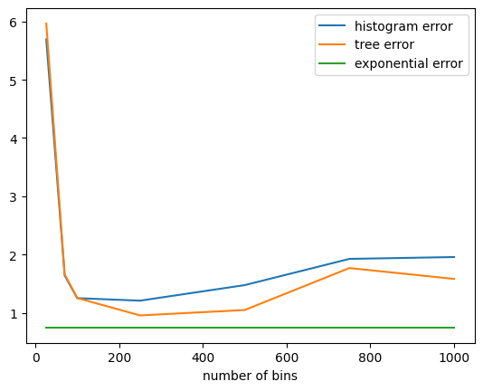
Of the three algorithms, when only estimating three quantiles, the exponential mechanism performs the best. However, the error will increase in the number of estimated quantiles more rapidly for the exponential mechanism than in the CDF-based mechanisms.

The utility of the tree-based algorithm is typically better than the histogram algorithm, and makes the algorithm less sensitive to the number of bins. In these simulations, the heuristic for picking the number of bins (25) was not helpful.

Privately Estimating the Distribution

Instead of postprocessing the noisy counts into quantiles, they can be left as counts, which can be used to visualize the distribution.

def make_distribution_counts(edges, scale):
    bin_names = [str(i) for i in range(len(edges - 1))]

    return (
        input_space >>
        dp.t.then_find_bin(edges=edges) >> # bin the data
        dp.t.then_index(bin_names, "0") >> # can be omitted. Just set TIA="usize", categories=list(range(num_bins)) on next line:
        dp.t.then_count_by_categories(categories=bin_names, null_category=False) >>
        dp.m.then_laplace(scale)
    )

edges = np.linspace(*bounds, num=50)
counts = make_distribution_counts(edges, scale=1.)(data)

import matplotlib.pyplot as plt

plt.hist(range(len(edges)), edges, weights=counts, density=True)
plt.xlabel("support")
plt.ylabel("noisy density");

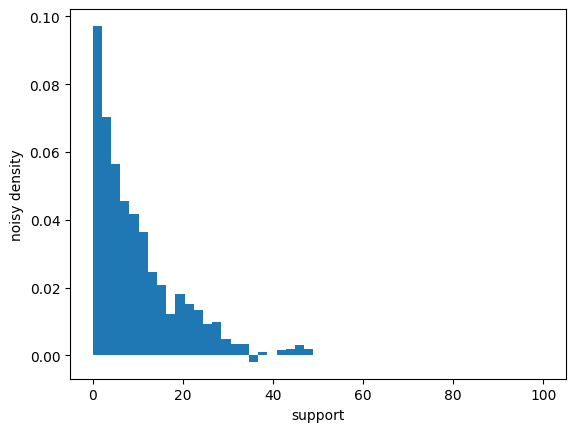
While the utility is not as great as the exponential mechanism, the histogram and tree approaches give more information about the distribution of the data.